LSTM forecasting horizontal line with standardized datas

[iMehqo]

Hello everyone,

I’ve seen many topics about the problem I have in my situation but nothing help.
I am trying to make a forecast on a stock price with a Bidirectional LSTM.
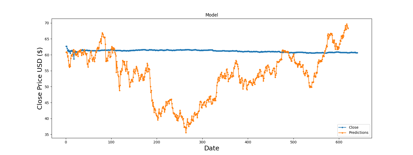
My problem here is that the forecast on test datas looks like almost horizontal during the whole period.
My data are standardized, and I tried to increase the number of epochs (actual is 300, but I tried 2000 and i got only nan values in prediction which seems to be caused by Exploding gradents).
Can you explain me if I made something wrong in my code ? I’ve been working on this since a week and cannot understand where am I wrong.

Thanks you a lot !!!

My code and final output :

!pip install yfinance

For reading stock data from yahoo

from pandas_datareader.data import DataReader
import yfinance as yf

import pandas as pd
import numpy as np

For time stamps

from datetime import datetime,timedelta

import matplotlib.pyplot as plt
import seaborn as sns
end = datetime.now()
print (‘end’,end)

start = “1900-01-01”
print(start)
print (‘start’,start)
globals()[‘SGO’] = yf.download(‘SGO.PA’, start, end,progress=False)
globals()[‘SGO’]=globals()[‘SGO’].filter([‘Close’])
symbols=‘SGO’
dic_train_len={}
data_array={}
data_array[symbols] = globals()[symbols].values
dic_train_len[symbols] = int(np.ceil( len(data_array[symbols]) * .90))
from sklearn.preprocessing import StandardScaler

Créer un dictionnaire pour stocker les scalers

dictio_scalers = {}

Fonction pour scaler un ensemble de données et conserver l’objet scaler

def scale_data(nom_symbole, dataset):
scaler = StandardScaler()
scaled_data = scaler.fit_transform(dataset)
dictio_scalers[nom_symbole] = scaler
return scaled_data

dictio_scaled_values = {}
dataset = globals()[‘SGO’].values
dictio_scaled_values[‘SGO’] = scale_data(‘SGO’, data_array[‘SGO’])
from sklearn.model_selection import cross_val_score
from keras.models import Sequential
from keras.layers import Dense, LSTM , Bidirectional
import tensorflow as tf
from tensorflow.keras.callbacks import EarlyStopping

def preparation_train(df_scaled,pas,train_len):

train_data = df_scaled[0:int(train_len)]
# Split the data into x_train and y_train data sets
x_train = []
y_train = []

for i in range(window_size, len(train_data)):
    x_train.append(train_data[i-window_size:i, 0])
    y_train.append(train_data[i, 0])


# Convert the x_train and y_train to numpy arrays
x_train, y_train = np.array(x_train), np.array(y_train)

# Reshape the data
x_train = np.reshape(x_train, (x_train.shape[0], x_train.shape[1], 1))

return x_train,y_train

def preparation_test(df_scaled,pas,train_len):

    # Create the data sets x_test and y_test
df_test= df_scaled[train_len:, :]
x_test = []
y_test = []
for i in range(pas, len(df_test)):
    x_test.append(df_test[i-pas:i, 0])
    y_test.append(df_test[i, 0])

Convert the x_test and y_test to numpy arrays

x_test, y_test = np.array(x_test), np.array(y_test)

# Reshape the data
x_test = np.reshape(x_test, (x_test.shape[0], x_test.shape[1], 1))

return x_test,y_test

def create_model(pas):
model = Sequential()
model.add(Bidirectional(LSTM(units=128, activation=‘relu’, input_shape=(pas, 1),return_sequences=True)))
model.add(Bidirectional(LSTM(units=64, activation=‘relu’,return_sequences=True)))
model.add(Bidirectional(LSTM(units=32, activation=‘relu’)))
model.add(Dense(1))
return model
epochs = 300
batch_size = 256
window_size=60
model = create_model(window_size)
model.compile(optimizer=‘adam’, loss=‘mean_squared_error’)
x_train,y_train = preparation_train(dictio_scaled_values[‘SGO’],window_size,dic_train_len[‘SGO’])
model.fit(x_train, y_train, batch_size=batch_size, epochs=epochs,verbose=1)
fichier_modele = “SGO.h5”
model.save(fichier_modele)
from keras.models import load_model
def Backtesting_real(df,symbols,train_len,pas):

Pred_Array_Global=df[int(train_len)-pas:int(train_len)]
test=df[train_len:]
 # Get the models predicted price values
fichier_modele = f"{symbols}.h5"
model = load_model(fichier_modele)
scaler2=dictio_scalers[symbols]
Pred_Array_Global=scaler2.fit_transform(Pred_Array_Global)

for i in range(0,len(test)):
    Pred_Array_Global=np.array(Pred_Array_Global)
    Pred_Array=Pred_Array_Global[i:i+pas]
    # Convert the data to a numpy array
    Pred_Array = np.array(Pred_Array)

    
    # Reshape the data
    Pred_Array_Input = np.reshape(Pred_Array,(1,pas, 1 ))
    predictions = model.predict(Pred_Array_Input,verbose=0)

    Pred_Array_Global=np.append(Pred_Array_Global,predictions)
    

Pred_Array_Global=Pred_Array_Global.reshape(-1,1)
#pdb.set_trace()
Pred_Array_Global2 = scaler2.inverse_transform(Pred_Array_Global)
Pred_Array_Global2=Pred_Array_Global2[pas:]
rmse = np.sqrt(np.mean(((Pred_Array_Global2 - test) ** 2)))
print("RMSE de l'action",symbols,":", rmse)
test_data={}
test_data['Predictions'] = Pred_Array_Global2
test_data['Close']=test
#pdb.set_trace()
# Visualize the data
plt.figure(figsize=(16,6))
plt.title('Model')
plt.xlabel('Date', fontsize=18)
plt.ylabel('Close Price USD ($)', fontsize=18)
for k, v in test_data.items():
    plt.plot(range(1, len(v) + 1), v, '.-', label=k)
plt.legend(['Close', 'Predictions'], loc='lower right')
plt.savefig(f"Backtesting {symbols}.png")

Backtesting_real(data_array[‘SGO’],‘SGO’,dic_train_len[‘SGO’],60)

[Tim_Wolfe]

TensorFlow Solutions Architect

The issue you’re encountering with your Bidirectional LSTM model predicting almost horizontal lines could stem from various factors including but not limited to data preprocessing, model architecture, and training process. Here are some common areas to review and adjust:

1. Data Preprocessing: Ensure that your data is correctly preprocessed. Since you’re standardizing the data, verify that the scaler is fitted on the training set and then used to transform both the training and test sets to maintain consistency. Also, check your input sequences and labels to ensure they’re correctly aligned and representative of the problem you’re trying to solve.
2. Model Complexity: Your model might be too complex or too simple for the task. Experiment with the number of layers, units in each LSTM layer, and other architectural parameters. Sometimes reducing complexity helps in avoiding overfitting, which could lead to poor generalization on the test set.
3. Learning Rate and Optimizer: The choice of optimizer and learning rate can significantly affect training. If you haven’t already, consider using learning rate schedules or adaptive learning rate optimizers like Adam. Also, experiment with different learning rates.
4. Regularization: To combat overfitting, consider adding dropout layers or using L2 regularization in your LSTM layers.
5. Exploding Gradients: Since you encountered NaN values at higher epochs, it’s a sign of exploding gradients. Implement gradient clipping in your optimizer to prevent this.
6. Epochs and Early Stopping: While increasing epochs, ensure you’re not overfitting. Use early stopping with a patience parameter to halt training when the model’s performance on a validation set stops improving.
7. Batch Size: Experiment with different batch sizes to find the optimal size for your model and data. Sometimes smaller batch sizes lead to better generalization.
8. Sequence Length (Window Size): The window size of 60 might not be optimal. Try shorter or longer sequences to see if the model captures the patterns more effectively.
9. Evaluation Metric: Ensure you’re using appropriate evaluation metrics for your forecast. RMSE is common, but depending on your specific needs, you might want to consider others like MAE or MASE.
10. Model Predictions Post-processing: After you get the predictions, ensure the post-processing (like inverse scaling) is correctly applied to compare the forecasted results with the actual values accurately.

Review these areas in your implementation to diagnose and rectify the issue with the horizontal predictions.